Project overview
The goal in this project is to implement your own discrete probabilistic programming language. The skeleton code for the project is available on GitHub:
https://github.com/neuppl/disc
Note: This is the first time we are ever running this project, and there is quite a bit of new code! If you encounter issues (you almost certainly will), please feel free to raise those issues with the instructor on Slack, and to file GitHub issues.
Due date: The project is due Tuesday Oct. 20 at 11:59PM EST. If you require an extension, email the instructor.
Rubric: The project will be evaluated according to following rubric:
- 70% Correctness
- A score of 100% is given for this category if all included tests in the GitHub repository are passed.
- If not all tests pass, partial credit will be assigned according to the percentage of tests that are passed.
- 30% Final writeup
- Include solutions to the modeling exercises. These are graded on a pass/no-pass scale.
- Please give us some feedback for future iterations on this project.
What to turn in: On Canvas, turn in the following:
- A
.zipfile containing your project. We should be able to unzip this file and rundune buildin order to build. - A
.pdffile containing your solutions to the modeling exercises.
Questions: Please e-mail any questions about build setup or the assignment itself to Minsung at minsung AT ccs.neu.edu.
Syntax
The disc language is a simple PPL that consists purely of Boolean random values. The syntax is given as two inductively defined terms: expressions e and programs p. A program is simply a designated start expression with no free variables. It has the following syntax:
e ::=
   | x <- e; e
   | observe e; e
   | flip q                         // q is a rational value
   | if e then e else e
   | return e
   | true | false
   | e && e | e || e | ! e |
   | ( e )

p ::= e
So for instance, we can write the following program in disc:
x <- flip 0.6;
y <- flip 0.3;
observe x || y;
return x
This program flips two coins and observes the outcome of at least one of them to be true, then returns the posterior probability of coin x being true. The resulting posterior is:
Semantics
The semantics for the probabilistic terms associates each term with an unnormalized probability distribution It has the type $[[e]] : \texttt{Bool} \rightarrow [0, 1]$, and has the following inductive definition:
\[[\![\texttt{flip}~\theta]\!](v) = \begin{cases} \theta& \quad \text{if }v = T\\ 1-\theta& \quad \text{if }v = F\\ \end{cases}\] \[[\![\texttt{return}~e]\!](v) = \begin{cases} 1\quad& \text{if }v = [\![e]\!]\\ 0\quad& \text{otherwise}\\ \end{cases}\] \[[\![x \leftarrow e_1; e_2]\!](v) = \sum_{v'} [\![{e_1}]\!](v') \times [\![{e_2[x \mapsto v']}]\!](v)\] \[[\![\texttt{observe}~e_1; e_2]\!](v) = \sum_{\{v' \mid [\![{e_1}(v') = T\}]\!]} [\![{e_2}]\!](v)\]The semantics for non-probabilistic terms is standard. The semantic evaluation has type $[[e]]: \texttt{Bool}$ for closed terms.
These semantics give an unnormalized distribution. The main semantic object of interest is the normalized distribution, which is given by the normalized semantics:
\[[\![e]\!]_D(T) = \frac{[\![e]\!](T)}{[\![e]\!](T) + [\![e]\!](F) },\]defined analogously for the false case.
Inference
You will be required to implement two inference algorithms for this project: (1) exact inference by enumeration, and (2) knowledge compilation based inference.
Enumeration
For this section we will be implementing exact inference via exhaustive enumeration. We will be filling in the lib/enumerate.ml file. Your solution should implement the infer function in this file.
Enumeration can be described as a big-step relation $e \Downarrow (\alpha, \beta)$ where $\alpha$ is the unnormalized true probability and $\beta$ is the unnormalized false probability. The adequacy requirement that this relation should satisfy is, if $e \Downarrow (\alpha, \beta)$, then:
\[[\![ e ]\!]_D(T) = \frac{\alpha}{\alpha + \beta}\]This relation is described inductively:
\[\frac{}{\texttt{flip}~\theta \Downarrow (\theta, 1-\theta)}\] \[\frac{e_1 \Downarrow (\alpha_1, \beta_1) \quad e_2[x \mapsto T] \Downarrow (\alpha_2, \beta_2) \quad e_2[x \mapsto F] \Downarrow (\alpha_3, \beta_3)} {x \leftarrow e_1; e_2 \Downarrow (\alpha_1\alpha_2 + \beta_1\alpha_3, \alpha_1\beta_2 + \beta_1\beta_3 )}\] \[\frac{} {\texttt{observe}~F; e_2 \Downarrow (0, 0)}\] \[\frac{e_1 \Downarrow (\alpha, \beta)} {\texttt{observe}~T; e_2 \Downarrow (\alpha, \beta)}\]Hint: What kinds of expressions should go in the observe statements? In the bindings? What is the semantics of observe (flip 0.5)?
Knowledge compilation
For this section we will be implementing exact inference via knowledge compilation. We will be filling in the lib/kc.ml file. Your solution should implement the infer function in this file. Knowledge compilation can be described as a big-step relation $e \Downarrow (\varphi, \gamma, w)$ where $\varphi$ and $\gamma$ are Boolean formulae and $w$ is a weight function. The invariant that these Boolean formulae should satisfy is that, for $e \Downarrow (\varphi, \gamma, w)$ the following holds:
The compilation relation is as follows:
\[\frac{\texttt{fresh variable }\ell}{\texttt{flip}~\theta \Downarrow (\ell, T, [\ell \mapsto \theta, \overline{\ell}\mapsto 1-\theta])}\] \[\frac{g \Downarrow (\varphi_g, \gamma_g, w_g) \quad t \Downarrow (\varphi_t, \gamma_t, w_t) \quad e \Downarrow (\varphi_e, \gamma_e, w_e)}{\texttt{if}~g~\texttt{then}~t~\texttt{else}~e \Downarrow ((\varphi_g \land \varphi_t) \lor (\neg\varphi_g \land \varphi_e), (\varphi_g \land \gamma_t) \lor (\neg\varphi_g \land \gamma_e), w_g \cup w_t \cup w_e)}\] \[\frac{e_1 \Downarrow (\varphi_1, \gamma_1, w_1) \quad e_2 \Downarrow (\varphi_2, \gamma_2, w_2)} {x \leftarrow e_1; e_2 \Downarrow (\varphi_2[x \mapsto \varphi_1], \gamma_2[x \mapsto \gamma_1], w_1 \cup w_2)}\]To build Boolean formulas and weight functions, we will be using the rsdd library. See a tutorial here.
Modeling exercises
The Monty Hall Problem
The Monty Hall problem is a classic “paradox” in probability theory. Here’s a shamelessly stolen Wikipedia description of the dilemma:
Suppose you’re on a game show, and you’re given the choice of three doors: Behind one door is a car; behind the others, goats. You pick a door, say No. 1, and the host, who knows what’s behind the doors, opens another door, say No. 3, which has a goat. He then says to you, “Do you want to pick door No. 2?” Is it to your advantage to switch your choice?
Your task is to make several .disc files that answers the host’s question for you:
-
In a file named
3doors.disc, make adiscprogram that represents the scenario in which you pick Door No. 1 before the host opens Door No. 3. The program should output the probability of winning the car. Make sure you can’t open two doors at once (we’ll be testing for that!). -
In a file named
no_switch.disc, make adiscprogram representing the scenario immediately after the host reveals a goat behind Door No. 3. The program should output the probability of winning the car provided we do not switch. -
In a file named
yes_switch.disc, make adiscprogram representing the scenario immediately after the host reveals a goat behind Door No. 3. The program should output the probability of winning the car provided we do switch.
Hint: If your program output for no_switch.disc or yes_switch.disc is 0.5 then it is wrong.
Network Reliability
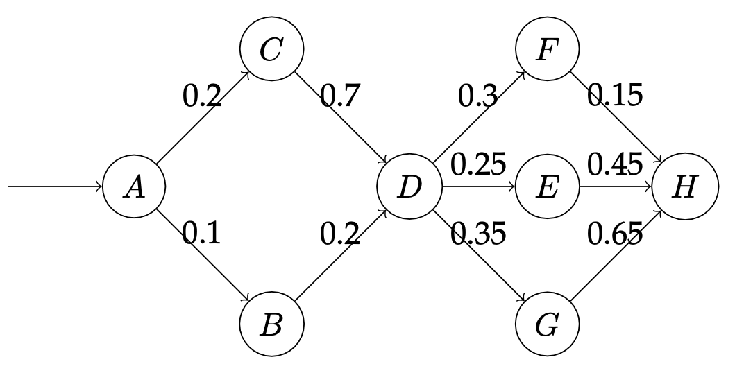
The directed graph above gives an abstract view of a computer network. The goal in a network like this is to deliver a packet – piece of data – from one router to another by passing it through intermediate routers in the graph. Each node is a router, and each directed edge is a link from one router to another. Packets always begin at $A$.
In the real world there is often some uncertainty in the behavior of such a network. Assume that each link has a failure probability given by its annotation; for instance, the probability that a packet traversing the link $A \rightarrow C$ fails to be delivered is 0.2. Furthermore, assume that, when given multiple options, a router will choose uniformly at random which router to forward to; for instance, if the packet is at node $A$, then at the next step it will have a 50% chance of being at node $C$ and a 50% chance of being at node $B$. Use your disc implementation and exact inference to answer the following questions about this network’s behavior:
- What is the probability that a packet successfully reaches $H$? Include your
discfile in the report. - If packet reached $H$, what is the probability that the packet reached $C$? Include your
discfile in the report. - If the packet did not reach $F$ or $G$, what is the probability that it reached $D$?
- Suppose I can fix a single edge to never drop a packet. Which edge should I fix to maximize the probability that a packet reaches $H$, and what is the probability that $H$ is reached in this new fixed network?
Extensions
For your final course project you may choose to extend disc in some way. Here are some suggestions for how to improve or extend disc:
- Develop and benchmark compiler optimizations.
- Extend
discto handle bounded and possibly unbounded loops.